一、数据基本情况

巴西公共电商数据共包含9张数据表，包含2016年至2018年，产生的订单数据，数据有十万条数据
一、 数据基本情况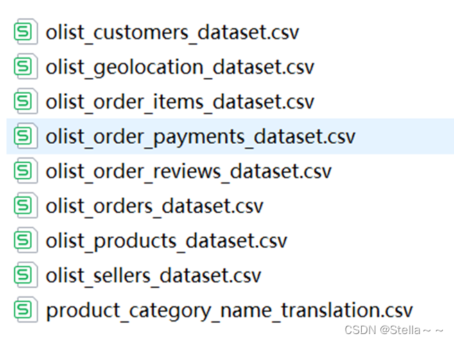

具体数据集含义：

表名	解释
Olist_customers_dataset	客户及其位置信息
Olist_geolocation_dataset	巴西邮政编码及其经纬度坐标信息
Olist_order_items_dataset	每个订单中购买的商品的数据
Olist_order_payments_dataset	订单付款的数据
Olist_order_reviews_dataset	客户所作评论数据
Olist_orders_dataset	订单交易数据
Olist_products_dataset	产品数据
Olist_sellers_dataset	完成订单的卖家的数据
Olist_category_name_translation	将商品从葡萄牙语转换为英语

二、数据清洗

使用python导入数据，查看数据中的缺失值，确定数据中的缺失值是否是重要的字段，若是补全，若不是，无影响可删除，或者忽略即可
格式检查，为了后续操作顺利，检查字段中的格式是否一致，不一致需要更改
去重，对于重复字段可以去重，去重一般在数据清洗之后进行，避免因为格式问题导致遗漏

查看数据表中数据基本情况
客户基本信息表（包含字段：订单对应的客户id，用户唯一id，客户所在地邮编号码，客户所在城市，所在州）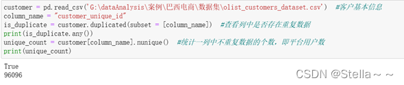

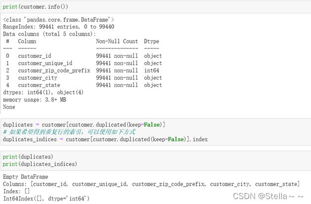
客户基本信息表包含99441条数据，5个字段，没有缺失值，没有重复行，通过统计平台中用户的唯一id
订单表（包含字段：订单id，产品识别同一订单中包含的项目数，商品id，商家id，卖家发货限制日期，商品价格，运费）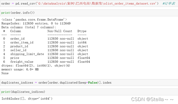

订单表共包含112650条数据，无重复值，无缺失值
支付表（包含字段：订单id，付款顺序，付款方式，客户选择分付款数量，交易金额）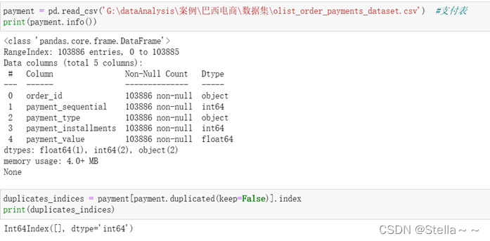

支付表中共103886条字段，无缺失值
评价表（包含字段：订单id，评价id，评价得分，评价标题，评价内容，发出满意度调查时间，客户满意度回复日期）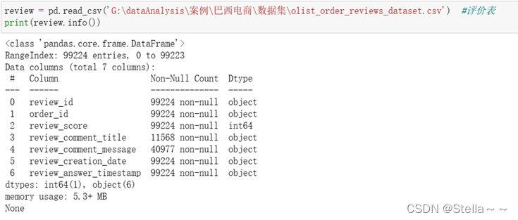

评价表中共包含99224条数据，其中评价标题和评价内容存在空值

订单交易数据（包含字段：包含订单id，订单对应的用户id，订单状态，下单时间，付款审批时间，订单过款时间，客户实际订单交货日期，订单预计交货日期）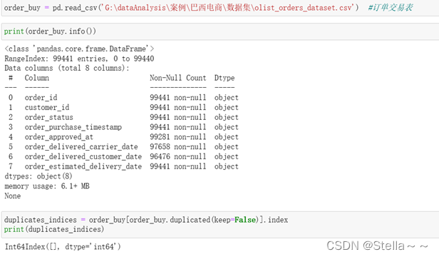

订单交易表中共包含99441条数据，其中订单审批时间，订单过款时间，客户实际订单交货日期存在缺失值

产品数据（包含字段：商品id，类别名称，产品名称长度，产品说明长度，产品招聘数量，产品重量，产品长度，产品高度，产品宽度）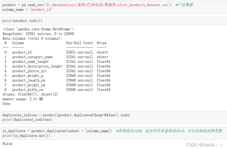

数据集中共包含32951条数据，除产品id外其余数据全部存在缺失值
商家数据（包含字段：商家id，商家所在地邮编号码，商家所在城市，所在州）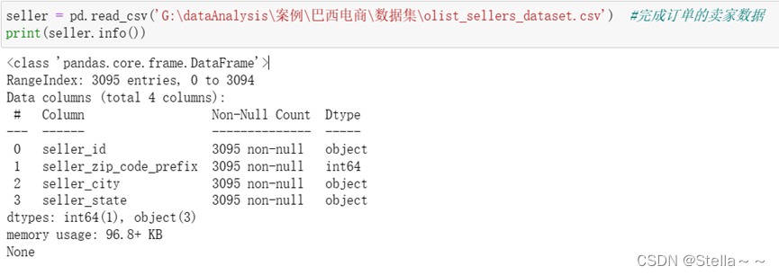


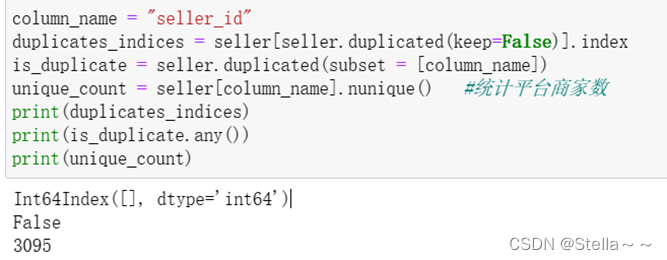
数据集一共包含3095条数据，无缺失值，无重复值
将商品从葡萄牙语转换为英语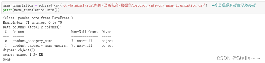

3.建立指标

按照“人”，“货”，“场”建立指标，如下：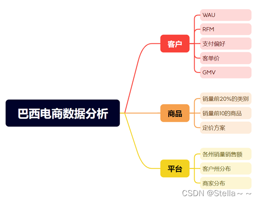

4.可视化分析

4.1 客户

支付偏好

select count(payment_type),payment_type
from olist.olist_order_payments_dataset
group by payment_type ;

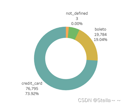
该平台客户的支付时喜欢信用卡和boleto支付（打印boleto小票，再到合作机构现金支付，类似线下“花呗”），结合客户占比及州单量和销售额占比，平台可以在SP,RJ,MG州结合用户的支付偏好，和相关支付平台合作策划促销活动

DAU

select count(distinct tt1.customer_unique_id) as DAU,tt1.paytime,tt1.customer_state
from (
select t1.customer_id, t1.order_status, t1.order_id, t1.paytime, t2.customer_unique_id,t2.customer_state
from (
select customer_id, substr(order_purchase_timestamp, 1, 10) paytime, order_id, order_status
from olist.olist_orders_dataset
where order_status in (‘delivered’, ‘invoiced’, ‘shipped’, ‘processing’, ‘created’, ‘approved’)
) t1
left join
(
select customer_id, customer_unique_id,customer_state
from olist.olist_customers_dataset
) t2
on t1.customer_id = t2.customer_id
) tt1
group by tt1.paytime,tt1.customer_state
order by tt1.paytime;

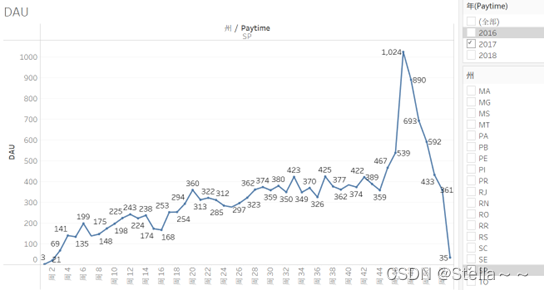
该平台WAU变化波动大，上图为SP州WAU，该平台用户活跃度变化较大

客单价

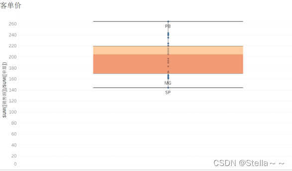
采用箱线图可视化客单价，从中可以看出SP，MG等州的客单价最低

GMV

RFM

select c.customer_unique_id,a.order_id,b.payment_value,substr(a.order_purchase_timestamp,1,10)
from olist.olist_orders_dataset a
left join olist.olist_order_payments_dataset b on a.order_id = b.order_id
left join olist.olist_customers_dataset c on a.customer_id = c.customer_id

计算字段

首先根据RFM对三个值的定义，计算RFM，在RFM模型中需要评分，需要将RFM标准化，采用归一化，即X = X-Xmin / Xmax -Xmin ,还需要设置RFM的参考值，将中位数设置为参考值，将标准化的RFM值和RFM的参考值对比大小，最后根据RFM对客户的划分，将客户划分为8类，逻辑如下：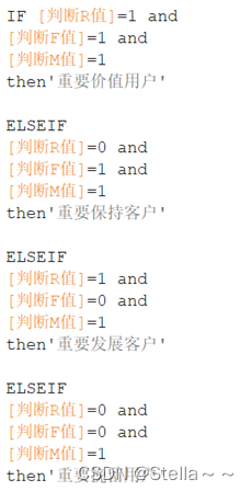



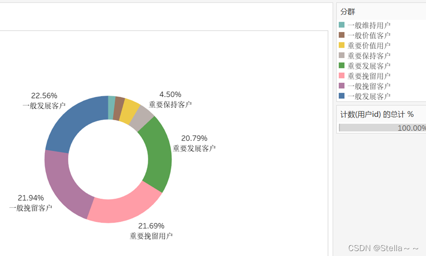
制定策略：
制定策略：对于重要价值客户，重要挽留客户，重要发展客户，因为其在平台产生过高额消费，可以制定相关的促销打折活动，进行客户召回
对于重要保持客户，一般保持客户，一般挽留客户，需要在控制运营成本内的适当展开促销，实现召回
对于其他的两种客户，因价值低，可在有多余的营销费用时进行召回

4.2商品

类别前20%销售额销量

– 查类别前20%销售额和销量
with df_1 as (
select t1.product_category_name,
sum(t2.payment_value) GMV,
count(t2.order_id) count_order,
dense_rank() over (order by sum(t2.payment_value) desc) rk
from (
select product_id, product_category_name
from olist.olist_products_dataset
) t1
left join
(
select a.product_id,
– a.price,
a.seller_id,
b.payment_value,
b.order_id
from olist.olist_order_items_dataset a
left join olist.olist_order_payments_dataset b on a.order_id = b.order_id
) t2
on t1.product_id = t2.product_id
group by t1.product_category_name
)
select * from df_1
where df_1.rk <=
( select max(rk) from df_1) * 0.2

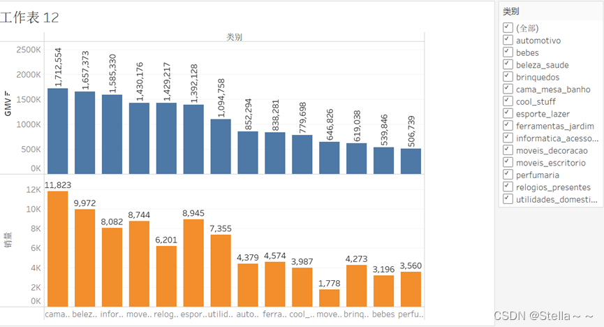
在前20%的品类中，cama_mesa_banho（生活用品）的销售额和销量是最高的

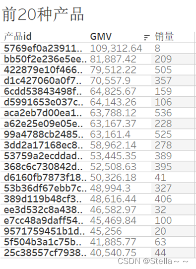
前20种产品销量销售额

– 因产品种类多，取1%仍有244种商品，因此取前20种

select t1.product_category_name,

select t1.product_id,
sum(t2.payment_value) GMV,
count(t2.order_id) count_order,
dense_rank() over (order by sum(t2.payment_value) desc) rk
from (
select product_id, product_category_name
from olist.olist_products_dataset
) t1
left join
(
select a.product_id,
– a.price,
a.seller_id,
b.payment_value,
b.order_id
from olist.olist_order_items_dataset a
left join olist.olist_order_payments_dataset b on a.order_id = b.order_id
) t2
on t1.product_id = t2.product_id

group by t1.product_category_name

group by t1.product_id
limit 20;

相关性分析

销量与评分

with df_1 as
(
select count(distinct tt1.order_id) 销量
, tt1.review_score
, tt1.seller_id
, tt1.product_category_name
, rank() over (order by count(distinct tt1.order_id) desc) rk
from (
select t1.order_id,
t1.product_id,
t1.seller_id,
t1.price,
t1.review_score,
t2.product_category_name
from (
select a.order_id, b.review_score, product_id, c.seller_id, c.price
from olist.olist_orders_dataset a
left join olist.olist_order_reviews_dataset b on a.order_id = b.order_id
left join olist.olist_order_items_dataset c on a.order_id = c.order_id
) t1
left join
(
select product_id, product_category_name
from olist.olist_products_dataset
) t2
on t1.product_id = t2.product_id
) tt1
group by tt1.review_score, tt1.product_category_name, tt1.seller_id
)
select df_1.product_category_name,df_1.seller_id,df_1.销量
,sum(case when df_1.review_score = 5 then 1 else 0 end) five
,sum(case when df_1.review_score = 4 then 1 else 0 end) four
,sum(case when df_1.review_score = 3 then 1 else 0 end) three
,sum(case when df_1.review_score = 2 then 1 else 0 end) two
,sum(case when df_1.review_score = 1 then 1 else 0 end) one

,row_number() over (partition by df_1.product_category_name order by df_1.price desc) as rk

from df_1
where df_1.rk <= (select max(rk) from df_1) * 0.2
group by df_1.product_category_name,df_1.销量,df_1.seller_id ;

销量与评分的相关性分析（python）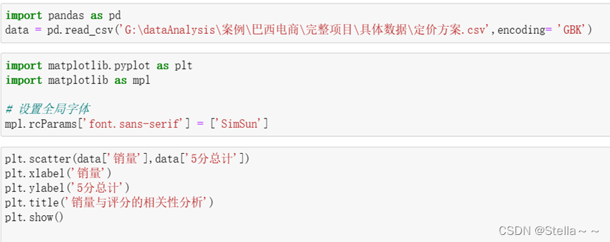



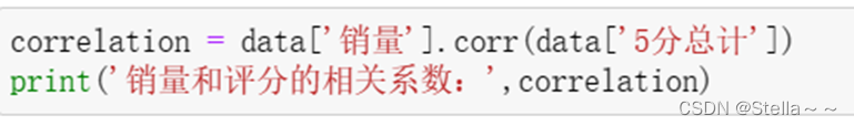
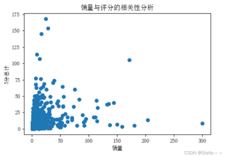
相关系数：销量和评分的相关系数： 0.3777695162799676
两个变量之间存在一定的正向相关性，但是相关性弱

销量与定价

销量与定价的相关性（python）

select count(distinct tt1.order_id) 销量
, tt1.seller_id
, tt1.price
, tt1.product_category_name
, rank() over (partition by tt1.seller_id,tt1.product_category_name order by tt1.price desc) rk
from (
select t1.order_id,
t1.product_id,
t1.seller_id,
t1.price,
t1.review_score,
t2.product_category_name
from (
select a.order_id, b.review_score, product_id, c.seller_id, c.price
from olist.olist_orders_dataset a
left join olist.olist_order_reviews_dataset b on a.order_id = b.order_id
left join olist.olist_order_items_dataset c on a.order_id = c.order_id
) t1
left join
(
select product_id, product_category_name
from olist.olist_products_dataset
) t2
on t1.product_id = t2.product_id
) tt1
group by tt1.product_category_name, tt1.seller_id,tt1.price

python计算中位数（因均值容易受极值影响，所以使用中位数来计算价格）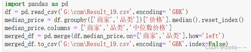

关联分析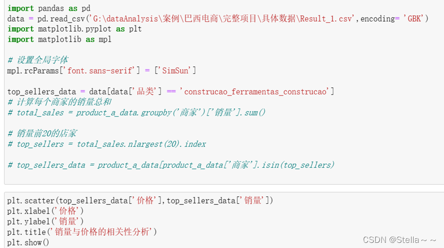



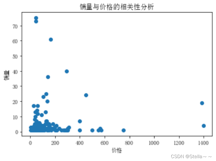
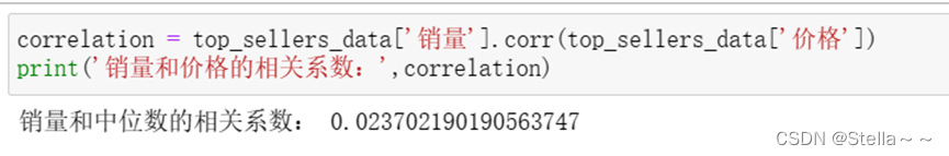
相关性较弱，可以参考销量高商家的定价，但仍需结合具体的市场情况

4.3 平台

客户州分布

select count(distinct customer_unique_id) as count_id
, customer_state
from olist.olist_customers_dataset
group by customer_state
order by count_id desc;

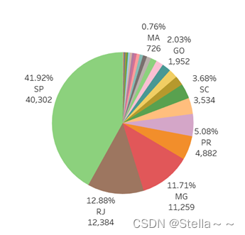
排名前三的是SP（圣保罗州）,RJ（里约热内卢州），MG（米纳斯吉拉斯州），占比达66.51%，是主要的客户来源

商家州分布

select count(distinct seller_id) as count_shop,seller_state
from olist.olist_sellers_dataset
group by seller_state
order by count_shop desc;

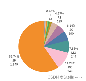
排名前三的是SP,PR(巴拉纳州)，MG，占比达78.9%，在客户分布中，RJ州占比达12.88%，排序第2，但商家占比排序第5，仅5.53%

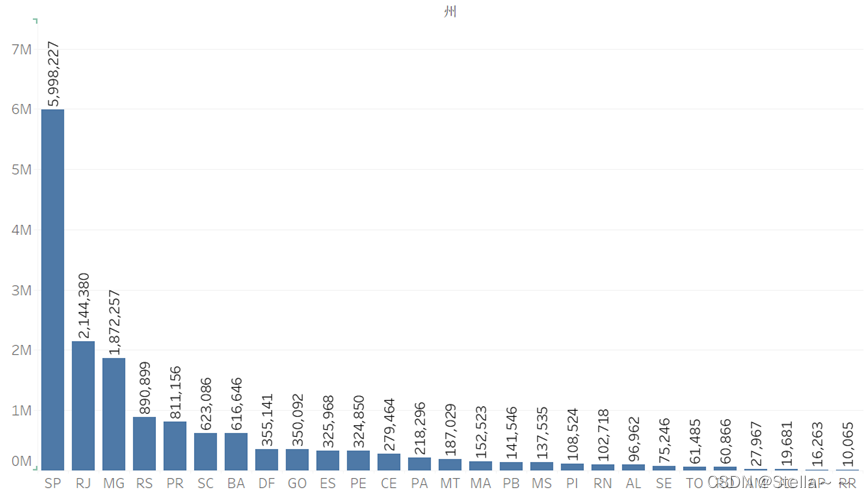
各州销售额销量排行

select count(distinct a.order_id) 单量,sum(a.payment_value) 销售额,c.customer_state 州
from olist.olist_order_payments_dataset a
left join olist.olist_orders_dataset b on a.order_id = b.order_id
left join olist.olist_customers_dataset c on b.customer_id = c.customer_id

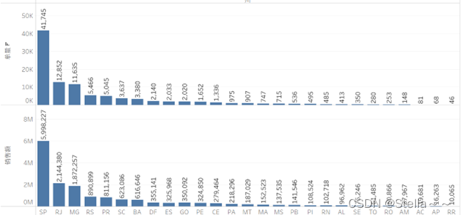
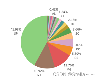
单量州分布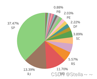

占比前三的仍是SP,RJ,MG州，这三个州的占比是主要的销量来源，可多次策划相关活动