本文是对上一篇博客的一些补充：
在第一到第二节中：介绍使用二进制定义传感器、通过对角定义传感器以及加载外部图像映射(将外部图像分配给初始压力分布，或理解为使用外部图像定义声源)三个方法，均基于官方的第一个示例：均匀传播介质(Example: Homogenous Propagation Medium)。
在第三节中：新增加了如何定义异构介质以及使用"kspaceFirstOrder2D"的内置绘图功能，基于官方示例：异构传播介质示例(Heterogeneous Propagation Medium Example)。

有兴趣的同好可以加企鹅群交流：937503951，任何科研相关问题都可以在群内交流，平常一起聊聊天、分享日常也是没问题的，欢迎~

目录

一、定义传感器

1.1 使用二进制定义传感器

1.2 通过对角定义传感器

1.3 注意事项

二、加载外部图像映射

三、定义异构介质并可视化

3.1 定义异构介质

3.2 使用内置绘图功能

一、定义传感器

1.1 使用二进制定义传感器

sensor_x_pos = Nx/2;        % [grid points] 
sensor_y_pos = Ny/2;        % [grid points] 
sensor_radius = Nx/2 - 22;  % [grid points] 
sensor_arc_angle = 3*pi/2;  % [radians]     
sensor.mask = makeCircle(Nx, Ny, sensor_x_pos, sensor_y_pos, sensor_radius, sensor_arc_angle);

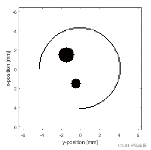
所绘制的传感器图如下，这时为一圈3/4圆的传感器，不再是用数量(50个)定义的传感器

1.2 通过对角定义传感器

% define the first rectangular sensor region by specifying the location of
% opposing corners
rect1_x_start = 25;
rect1_y_start = 31;
rect1_x_end = 30;
rect1_y_end = 50;

% define the second rectangular sensor region by specifying the location of
% opposing corners
rect2_x_start = 71;
rect2_y_start = 81;
rect2_x_end = 80;
rect2_y_end = 90;

% assign the list of opposing corners to the sensor mask
sensor.mask = [rect1_x_start, rect1_y_start, rect1_x_end, rect1_y_end;...
               rect2_x_start, rect2_y_start, rect2_x_end, rect2_y_end].';

rect1_x_start = 25; %x起始坐标：25*0.1=2.5[mm]，-6.4+2.5=-3.9[mm]
rect1_y_start = 31; %y起始坐标：-3.3[mm]
rect1_x_end = 30;  %x终止坐标：-3.4[mm]
rect1_y_end = 50;  %y终止坐标：-1.4[mm]
% 上面所绘制的矩形为较扁的那一个，另一个矩形同理
% assign the list of opposing corners to the sensor mask
sensor.mask = [rect1_x_start, rect1_y_start, rect1_x_end, rect1_y_end;...
                         rect2_x_start, rect2_y_start, rect2_x_end, rect2_y_end].';
% sensor.mask也不再是用函数"makeCartCircle"或"makeCircle"赋值
% 这里是将对角列表(矩阵)分配给"sensor.mask"，可以通过添加额外的列向量来指定多个矩形。

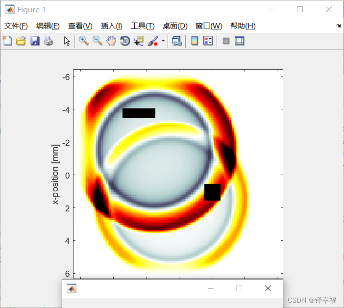
定义传感器所用的矩形区域见下图中黑色长方形：

1.3 注意事项

注：以上两种方法在输出数据、数据可视化时，与原官方示例中(均匀传播介质)的书写的程序有所不用，具体见官方示例中的解释。

二、加载外部图像映射

此部分演示了如何将外部图像分配给初始压力分布(或理解为：使用外部图像定义声源)，以模拟二维均匀传播介质中的初始值问题。

原官方示例中的"kspaceFirstOrder2D"使用的初始压力分布"source.p0"只是一个填充了任意数值的二维矩阵。因此，任何数据都可以用来定义这种分布。

% load the initial pressure distribution from an image and scale the magnitude
p0_magnitude = 3;
p0 = p0_magnitude * loadImage('EXAMPLE_source_one.png');
% resize the image to match the size of the computational grid and assign
% to the source input structure
source.p0 = resize(p0, [Nx, Ny]);

p0 = p0_magnitude * loadImage('EXAMPLE_source_one.png');
% 这里使用"loadImage"加载外部图像映射。
% 使用的外部图像名为"EXAMPLE_source_one.png"，此图片和官方示例文件(.m)放在同一个目录下。
% 该函数将外部图像转换为矩阵，对颜色通道(用于彩色图像)求和，并将像素值从0缩放到1。
source.p0 = resize(p0, [Nx, Ny])
% 调整图像大小，以匹配计算网格的大小并分配给源输入结构。
% 原方法使用的是：source.p0 = disc_magnitude * makeDisc(Nx, Ny, disc_x_pos, disc_y_pos, disc_radius);

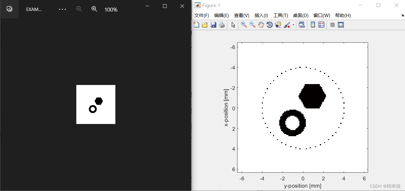
外部图像及此方式下的初始压力分布图如下：

注：此方法在输出数据、数据可视化时，书写程序与原官方示例基本一致，无需过多调整。

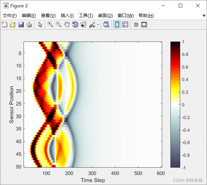
可视化结果如下：

三、定义异构介质并可视化

注：以下程序来自于官方示例：异构传播介质示例

3.1 定义异构介质

对于均匀传播介质，声速被指定为单位制单位的单个标量值。
如果传播介质是异质的，"sound_speed"和"medium.density"是作为与计算网格(即Nx行和Ny列)具有相同维度的矩阵给出的。
这些矩阵可以以几种方式创建：包括直接定义(如下所示)、从外部图像映射、或使用来自其他模拟或实验成像模式的空间或体积数据。

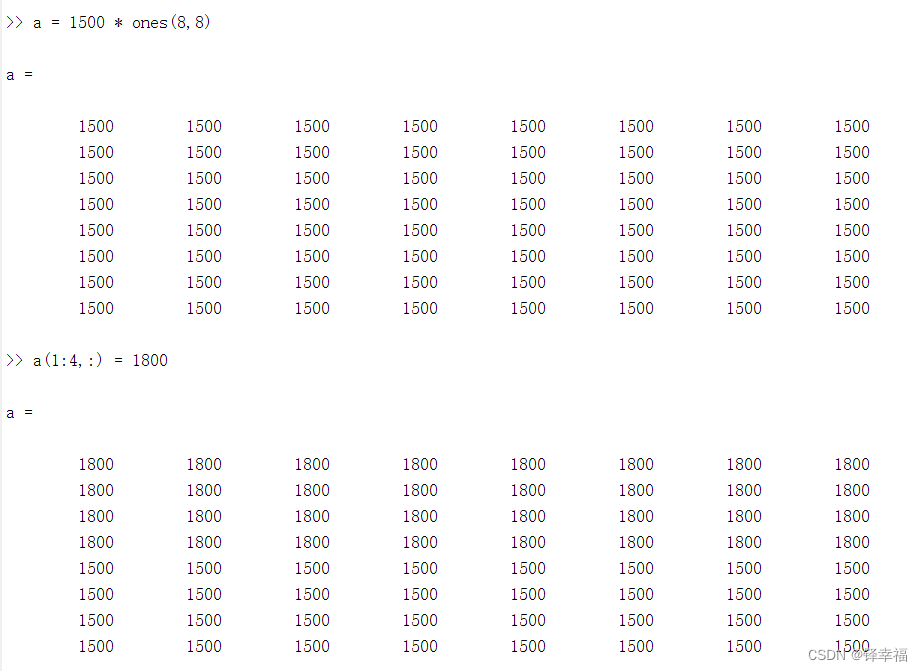
% define the properties of the propagation medium    
medium.sound_speed = 1500 * ones(Nx, Ny);   % [m/s]
medium.sound_speed(1:Nx/2, :) = 1800;       % [m/s]
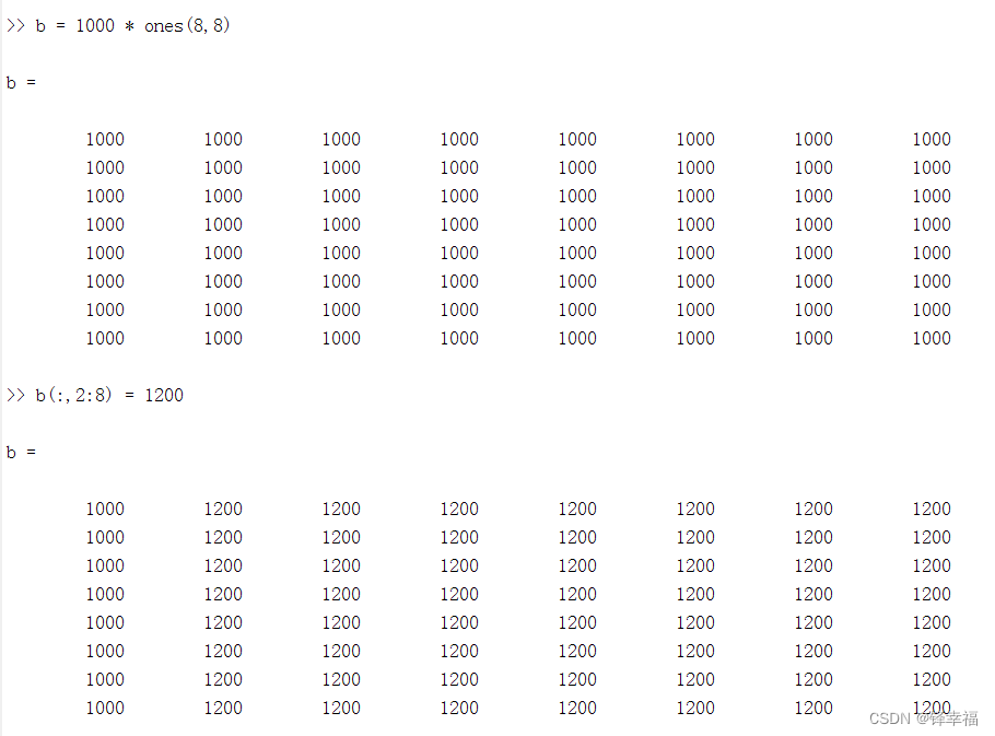
medium.density = 1000 * ones(Nx, Ny);       % [kg/m^3]
medium.density(:, Ny/4:Ny) = 1200;          % [kg/m^3]

medium.sound_speed = 1500 * ones(Nx, Ny);  % [m/s]
% "ones"为创建全为1的矩阵，此时"medium.sound_speed"为128行128列全为1500的矩阵
medium.sound_speed(1:Nx/2, :) = 1800;       % [m/s]
% 将上述矩阵，1到64行的全部列中的数字1500都变为1800
medium.density = 1000 * ones(Nx, Ny);       % [kg/m^3]
% "medium.density"为128行128列全为1000的矩阵
medium.density(:, Ny/4:Ny) = 1200;          % [kg/m^3]
% 将上述矩阵，32到128列的全部行中的数字1000都变为1200

下面给出小例子方便理解上述程序：

3.2 内置绘图功能

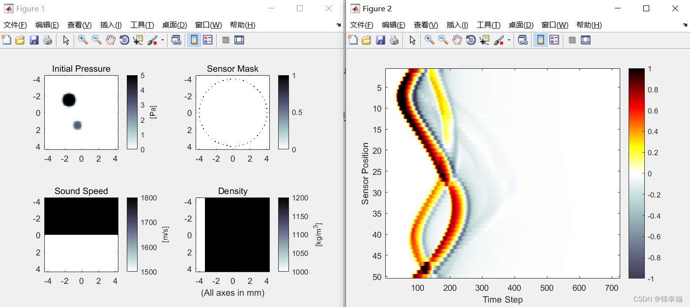
除了使用"imagesc"函数进行绘图外，还可以使用"kspaceFirstOrder2D"的内置绘图功能：

% run the simulation with optional inputs for plotting the simulation
% layout in addition to removing the PML from the display
sensor_data = kspaceFirstOrder2D(kgrid, medium, source, sensor, ...
    'PlotLayout', true, 'PlotPML', false);

通过输入“PlotLayout”设置为"true"，即可使用"kspaceFirstOrder2D"的内置绘图功能；这里将"PlotPML"设置为"false"，关闭PML(完美匹配层)的显示。

可视化结果如下：（与均匀传播介质相比，主波前的形状受到了扰动，并且还可以看到来自非均匀界面的弱反射）